an encyclopedia of finite element definitions
How to define a finite element
↓ Cite this page ↓This page describes how finite elements are defined in the DefElement database.
Cell subentities
Throughout this website, the subentities of a reference element will be referred to as described here.
The vertices, edges, faces, and volumes of a reference element have dimension 0, 1, 2, and 3 (respectively). The (topological) dimension \(d\) is the dimension of the reference element itself. (When using the finite element method, the topological dimensions may differ from the geometric dimension: for example, when meshing a 2D manifold in 3D space, the topological and geometric dimensions are 2 and 3 (respectively).)
The codimension of an entity is given by subtracting the dimension of the entity from the topological dimension of the reference element. Entities of codimension 1, 2, and 3 are called facets, ridges and peaks (respectively). The usual names given to entities of reference elements of topological dimensions 0 to 3 are shown below.
| Topological dimension | Entities by dimension | Entities by codimension | ||||||
| 0 | 1 | 2 | 3 | 0 | 1 (facets) | 2 (ridges) | 3 (peaks) | |
| 0 (a vertex) | point | - | - | - | cell | - | - | - |
| 1 (an interval) | points | edge | - | - | cell | points | - | - |
| 2 (a polygon) | points | edges | face | - | cell | edges | points | - |
| 3 (a polyhedron) | points | edges | faces | volume | cell | faces | edges | points |
Ciarlet finite elements
The Ciarlet definition[1] defines a finite element by a triple \((R,\mathcal{V},\mathcal{L})\), where
- \(R\subset\mathbb{R}^d\) is the reference element, usually a polygon or polyhedron;
- \(\mathcal{V}\) is a finite dimensional polynomial space on \(R\) of dimension \(n\);
- \(\mathcal{L}=\{l_0,...,l_{n-1}\}\) is a basis of the dual space \(\mathcal{V}^*=\{f:\mathcal{V}\to\mathbb{R}|f\text{ is linear}\}\). Each functional \(l_i\) is associated with a subentity of the reference element \(R\).
The basis functions \(\{\phi_0,...,\phi_{n-1}\}\) of the finite element space are defined by
\[l_i(\phi_j) = \begin{cases}1&i=j\\0&i\not=j\end{cases}\]The correct continuity is enforced by ensuring that the same global degree-of-freedom is associated with corresponding functionals on the shared subentities of neighbouring cells.
Example: Order 1 Lagrange space on a triangle
An order 1 Lagrange space on a triangle is defined by:
- \(R\) is a triangle with vertices at \((0,0)\), \((1,0)\) and \((0,1)\);
- \(\mathcal{V}=\operatorname{span}\{1, x, y\}\);
- \(\mathcal{L}=\{l_0,l_1,l_2\}\).
The functionals \(l_0\) to \(l_2\) are defined as point evaluations at the three vertices of the triangle:
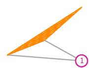
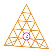
\[l_0:v\mapsto v(0,0)\] \[l_1:v\mapsto v(1,0)\] \[l_2:v\mapsto v(0,1)\]It follows from these definitions that the basis functions of the finite element spaces are linear functions that are equal 1 to at one of the vertices, and equal to 0 at the other two. These are:
\[\phi_0(x,y)=1-x-y\] \[\phi_1(x,y)=x\] \[\phi_2(x,y)=y\]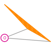
Integral moments
It is common to use integral moment functionals when defining finite elements. Given a mesh entity \(e\) and a finite element space \((e,\mathcal{V}_e,\mathcal{L}_e)\) defined on \(e\), the integral moment functionals \(l_1,...,l_{n_e}\) are defined by \[l_i:v\mapsto \int_e v\phi_i,\] where \(\phi_1,...,\phi_{n_e}\) are the basis functions of the finite element space on \(e\).
For vector-valued spaces, integral moment functional can be defined using a vector-valued space on \(e\) and taking the dot product inside the integral, \[l_i:\boldsymbol{v}\mapsto \int_e \boldsymbol{v}\cdot\boldsymbol{\phi}_i.\] Alternatively, an integral moment can be taken with a scalar-valued space by taking the dot product with a fixed vector \(\boldsymbol{a}\), \[l_i:\boldsymbol{v}\mapsto \int_e \boldsymbol{v}\cdot\boldsymbol{a}\,\phi_i.\] Typically, \(\boldsymbol{a}\) will be tangent to an edge, normal to a facet, or a unit vector in one of the coordinate directions.
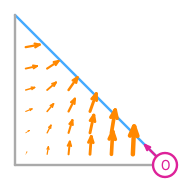
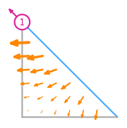
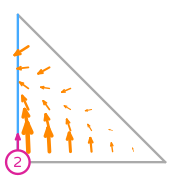
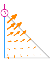
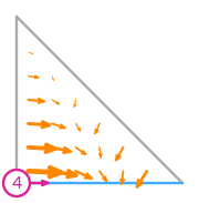
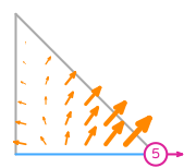
Example: Order 1 Nédélec (second kind) space on a triangle
The functionals that define an order 1 Nédélec (second kind) space on a triangle[2] are tangential integral moments with order 1 Lagrange spaces on the edges of the triangle. For example, the two functionals on the edge \(e_0\) of the triangle between \((1,0)\) and \((0,1)\) are \[l_0:\boldsymbol{v}\to\int_{e_0}\boldsymbol{v}\cdot\left(\begin{array}{c}-\frac1{\sqrt2}\\\frac1{\sqrt{2}}\end{array}\right)(1-s_0),\] \[l_1:\boldsymbol{v}\to\int_{e_0}\boldsymbol{v}\cdot\left(\begin{array}{c}-\frac1{\sqrt2}\\\frac1{\sqrt{2}}\end{array}\right)s_0,\] where \(s_0\) varies from 0 (at \((1,0)\)) to 1 (at \((0,1)\)) along \(e_0\).
The basis functions of this space are:
Mapping finite elements
In order to maintain desired properties when mapping finite elements from a reference element to an actual mesh, an appropriate mapping must be defined.[3][4] (For elements with a mixture of functional types, a more complex approach is required.[5])
Let \(F\) be a transformation that maps the reference element to a cell in the mesh, and let \(\boldsymbol{x}\) be a point in the cell.
The Jacobian, \(\mathbf{J}\), of the transformation \(F\) is \(\displaystyle\frac{\mathrm{d}F}{\mathrm{d}x}\) for 1D reference elements, \(\displaystyle\left( \begin{array}{cc} \frac{\partial F_1}{\partial x}&\frac{\partial F_1}{\partial y}\\ \frac{\partial F_2}{\partial x}&\frac{\partial F_2}{\partial y} \end{array} \right)\) for 2D reference elements, or \(\displaystyle\left( \begin{array}{ccc} \frac{\partial F_1}{\partial x}&\frac{\partial F_1}{\partial y}&\frac{\partial F_1}{\partial z}\\ \frac{\partial F_2}{\partial x}&\frac{\partial F_2}{\partial y}&\frac{\partial F_2}{\partial z}\\ \frac{\partial F_3}{\partial x}&\frac{\partial F_3}{\partial y}&\frac{\partial F_3}{\partial z} \end{array} \right)\) for 3D reference elements.
Scalar-valued basis functions
The simplest mapping—used to map scalar basis functions, \(\phi\)—is defined by $$\left(\mathcal{F}\phi\right)(\boldsymbol{x}) :=\phi(F^{-1}(\boldsymbol{x})).$$ The term \(F^{-1}(\boldsymbol{x})\) is the point on the reference element corresponding to the point \(\boldsymbol{x}\), so this mapping maps a value of the function on the reference to the same value at the corresponding point.
Vector-valued basis functions
For vector-valued basis functions, \(\boldsymbol{\phi}\), the covariant Piola (\(\mathcal{F}^\text{curl}\)) and contravariant Piola (\(\mathcal{F}^\text{div}\)) mappings are defined: $$\left(\mathcal{F}^\text{curl}\boldsymbol{\phi}\right)(\boldsymbol{x}) :=\mathbf{J}^{-T}\boldsymbol{\phi}(F^{-1}(\boldsymbol{x}))$$ $$\left(\mathcal{F}^\text{div}\boldsymbol{\phi}\right)(\boldsymbol{x}) :=\frac1{\det \mathbf{J}}\mathbf{J}\boldsymbol{\phi}(F^{-1}(\boldsymbol{x}))$$ The covariant Piola mapping preserves the tangential component of basis functions on edges and facets, and are typically used to map H(curl) elements. The contravariant Piola mapping preserves the normal component of basis functions on facets, and are typically used to map H(div) elements.
Matrix-valued basis functions
For matrix-valued basis functions, \(\mathbf{\Phi}\), the double covariant Piola (\(\mathcal{F}^\text{curl curl}\)) and double contravariant Piola (\(\mathcal{F}^\text{div div}\)) mappings are defined: $$\left(\mathcal{F}^\text{curl curl}\mathbf{\Phi}\right)(\boldsymbol{x}) :=\mathbf{J}^{-T}\mathbf{\Phi}(F^{-1}(\boldsymbol{x}))\mathbf{J}^{-1}$$ $$\left(\mathcal{F}^\text{div div}\mathbf{\Phi}\right)(\boldsymbol{x}) :=\frac1{\left(\det \mathbf{J}\right)^2}\mathbf{J}\mathbf{\Phi}(F^{-1}(\boldsymbol{x}))\mathbf{J}^T$$
Variants of finite elements
For many elements, there are a number of different choices that could be made for the functionals in \(\mathcal{L}\) that define the element that give rise to an element with the same key properties. For example, when defining a Lagrange element on a triangle, there are many possible choices for where exactly to locate the point evaluation functionals. We refer to a pair of elements as variants of each other if:
- They are defined on the same reference element \(R\);
- They are defined using the same polynomial set \(\mathcal{V}\);
- The functionals in \(\mathcal{L}\) associated with each facet, ridge, and peak of the cell, and the push forward/pull back map used lead to the same type of continuity between cells.
Commonly used variants of elements are shown on each element's page.
The degree of a finite element
There are a few different ways to describe the (polynomial) degree of a finite element:
- The polynomial subdegree is the degree of the highest degree complete polynomial space that is a subspace of this element's polynomial space.
- The polynomial superdegree is the degree of the lowest degree complete polynomial space that is a superspace of this element's polynomial space.
- The Lagrange subdegree is the degree of the highest degree Lagrange space that is a subspace of this element's polynomial space.
- The Lagrange superdegree is the degree of the lowest degree Lagrange space that is a superspace of this element's polynomial space.
On each element's page, the value of these is shown, as well as information about which one is used as the canonical degree of that element.
Notation
Throughout this website, the notation given here in this section is used.
| \(R\) | A reference element |
| \(\mathcal{V}\) | A polynomial set |
| \(\mathcal{L}\) | A dual basis |
| \(l_i\) | A functional in the dual basis |
| \(\phi_i\) | A scalar basis function |
| \(\boldsymbol{\phi}_i\) | A vector basis function |
| \(\mathbf{\Phi}_i\) | A matrix basis function |
| \(\mathbf{J}\) | Jacobian |
| \(F\) | A map from a reference to a cell in a mesh |
| \(\mathcal{F}\) | A mapping |
| \(v_i\) | The \(i\)th vertex |
| \(e_i\) | The \(i\)th edge |
| \(f_i\) | The \(i\)th face |
| \(c_i\) | The \(i\)th volume |
| \(k\) | Degree of a finite element |
| \(d\) | Geometric dimension |
| \(r\) | Exterior derivative order |
References
- [1] Ciarlet, P. G. The Finite Element Method for Elliptic Problems, 1978.
- [2] Nédélec, J. C. A new family of mixed finite elements in \(\mathbb{R}^3\), Numerische Mathematik 50(1), 57–81, 1986. [DOI: 10.1007/BF01389668]
- [3] Rognes, M. E. and Kirby, R. C. and Logg, A. Efficient assembly of H(div) and H(curl) conforming finite elements, SIAM Journal on Scientific Computing 31, 4130–4151, 2009. [DOI: 10.1137/08073901X]
- [4] Arnold, D. A. and Boffi, D. and Falk, R. S. Quadrilateral H(div) Finite Elements, SIAM Journal on Numerical Analysis 42, 2429–2451, 2005. [DOI: 10.1137/S0036142903431924]
- [5] Kirby, R. C. A general approach to transforming finite elements, The SMAI journal of computational mathematics 4, 197–224, 2018. [DOI: 10.5802/smai-jcm.33]