an encyclopedia of finite element definitions
Degree 1 Tiniest tensor H(curl) on a quadrilateral
◀ Back to Tiniest tensor H(curl) definition page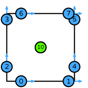
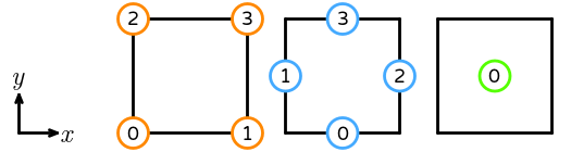
- \(R\) is the reference quadrilateral. The following numbering of the subentities of the reference is used:
- \(\mathcal{V}\) is spanned by: \(\left(\begin{array}{c}\displaystyle 1\\\displaystyle 0\end{array}\right)\), \(\left(\begin{array}{c}\displaystyle 0\\\displaystyle 1\end{array}\right)\), \(\left(\begin{array}{c}\displaystyle y\\\displaystyle 0\end{array}\right)\), \(\left(\begin{array}{c}\displaystyle 0\\\displaystyle y\end{array}\right)\), \(\left(\begin{array}{c}\displaystyle x\\\displaystyle 0\end{array}\right)\), \(\left(\begin{array}{c}\displaystyle 0\\\displaystyle x\end{array}\right)\), \(\left(\begin{array}{c}\displaystyle x y\\\displaystyle 0\end{array}\right)\), \(\left(\begin{array}{c}\displaystyle 0\\\displaystyle x y\end{array}\right)\), \(\left(\begin{array}{c}\displaystyle \frac{3 y \left(1 - y\right)}{2}\\\displaystyle 0\end{array}\right)\), \(\left(\begin{array}{c}\displaystyle 0\\\displaystyle \frac{3 x \left(x - 1\right)}{2}\end{array}\right)\), \(\left(\begin{array}{c}\displaystyle \frac{3 y \left(2 x y - 2 x - y + 1\right)}{2}\\\displaystyle \frac{3 x \left(- 2 x y + x + 2 y - 1\right)}{2}\end{array}\right)\)
- \(\mathcal{L}=\{l_0,...,l_{10}\}\)
- Functionals and basis functions:
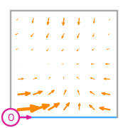
\(\displaystyle l_{0}:\boldsymbol{v}\mapsto\displaystyle\int_{e_{0}}\boldsymbol{v}\cdot(1 - s_{0})\hat{\boldsymbol{t}}_{0}\)
where \(e_{0}\) is the 0th edge;
\(\hat{\boldsymbol{t}}_{0}\) is the tangent to edge 0;
and \(s_{0},s_{1}\) is a parametrisation of \(e_{0}\).
\(\displaystyle \boldsymbol{\phi}_{0} = \left(\begin{array}{c}\displaystyle - 9 x y^{2} + 15 x y - 6 x + \frac{15 y^{2}}{2} - \frac{23 y}{2} + 4\\\displaystyle \frac{9 x \left(2 x y - x - 2 y + 1\right)}{2}\end{array}\right)\)
This DOF is associated with edge 0 of the reference element.
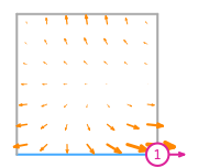
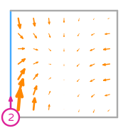
\(\displaystyle l_{1}:\boldsymbol{v}\mapsto\displaystyle\int_{e_{0}}\boldsymbol{v}\cdot(s_{0})\hat{\boldsymbol{t}}_{0}\)
where \(e_{0}\) is the 0th edge;
\(\hat{\boldsymbol{t}}_{0}\) is the tangent to edge 0;
and \(s_{0},s_{1}\) is a parametrisation of \(e_{0}\).
\(\displaystyle \boldsymbol{\phi}_{1} = \left(\begin{array}{c}\displaystyle 9 x y^{2} - 15 x y + 6 x - \frac{3 y^{2}}{2} + \frac{7 y}{2} - 2\\\displaystyle \frac{9 x \left(- 2 x y + x + 2 y - 1\right)}{2}\end{array}\right)\)
This DOF is associated with edge 0 of the reference element.
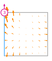
\(\displaystyle l_{2}:\boldsymbol{v}\mapsto\displaystyle\int_{e_{1}}\boldsymbol{v}\cdot(1 - s_{0})\hat{\boldsymbol{t}}_{1}\)
where \(e_{1}\) is the 1st edge;
\(\hat{\boldsymbol{t}}_{1}\) is the tangent to edge 1;
and \(s_{0},s_{1}\) is a parametrisation of \(e_{1}\).
\(\displaystyle \boldsymbol{\phi}_{2} = \left(\begin{array}{c}\displaystyle \frac{9 y \left(2 x y - 2 x - y + 1\right)}{2}\\\displaystyle - 9 x^{2} y + \frac{15 x^{2}}{2} + 15 x y - \frac{23 x}{2} - 6 y + 4\end{array}\right)\)
This DOF is associated with edge 1 of the reference element.
\(\displaystyle l_{3}:\boldsymbol{v}\mapsto\displaystyle\int_{e_{1}}\boldsymbol{v}\cdot(s_{0})\hat{\boldsymbol{t}}_{1}\)
where \(e_{1}\) is the 1st edge;
\(\hat{\boldsymbol{t}}_{1}\) is the tangent to edge 1;
and \(s_{0},s_{1}\) is a parametrisation of \(e_{1}\).
\(\displaystyle \boldsymbol{\phi}_{3} = \left(\begin{array}{c}\displaystyle \frac{9 y \left(- 2 x y + 2 x + y - 1\right)}{2}\\\displaystyle 9 x^{2} y - \frac{3 x^{2}}{2} - 15 x y + \frac{7 x}{2} + 6 y - 2\end{array}\right)\)
This DOF is associated with edge 1 of the reference element.
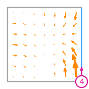
\(\displaystyle l_{4}:\boldsymbol{v}\mapsto\displaystyle\int_{e_{2}}\boldsymbol{v}\cdot(1 - s_{0})\hat{\boldsymbol{t}}_{2}\)
where \(e_{2}\) is the 2nd edge;
\(\hat{\boldsymbol{t}}_{2}\) is the tangent to edge 2;
and \(s_{0},s_{1}\) is a parametrisation of \(e_{2}\).
\(\displaystyle \boldsymbol{\phi}_{4} = \left(\begin{array}{c}\displaystyle \frac{9 y \left(2 x y - 2 x - y + 1\right)}{2}\\\displaystyle \frac{x \left(- 18 x y + 15 x + 6 y - 7\right)}{2}\end{array}\right)\)
This DOF is associated with edge 2 of the reference element.
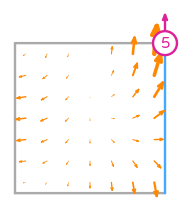
\(\displaystyle l_{5}:\boldsymbol{v}\mapsto\displaystyle\int_{e_{2}}\boldsymbol{v}\cdot(s_{0})\hat{\boldsymbol{t}}_{2}\)
where \(e_{2}\) is the 2nd edge;
\(\hat{\boldsymbol{t}}_{2}\) is the tangent to edge 2;
and \(s_{0},s_{1}\) is a parametrisation of \(e_{2}\).
\(\displaystyle \boldsymbol{\phi}_{5} = \left(\begin{array}{c}\displaystyle \frac{9 y \left(- 2 x y + 2 x + y - 1\right)}{2}\\\displaystyle \frac{x \left(18 x y - 3 x - 6 y - 1\right)}{2}\end{array}\right)\)
This DOF is associated with edge 2 of the reference element.
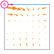
\(\displaystyle l_{6}:\boldsymbol{v}\mapsto\displaystyle\int_{e_{3}}\boldsymbol{v}\cdot(1 - s_{0})\hat{\boldsymbol{t}}_{3}\)
where \(e_{3}\) is the 3rd edge;
\(\hat{\boldsymbol{t}}_{3}\) is the tangent to edge 3;
and \(s_{0},s_{1}\) is a parametrisation of \(e_{3}\).
\(\displaystyle \boldsymbol{\phi}_{6} = \left(\begin{array}{c}\displaystyle \frac{y \left(- 18 x y + 6 x + 15 y - 7\right)}{2}\\\displaystyle \frac{9 x \left(2 x y - x - 2 y + 1\right)}{2}\end{array}\right)\)
This DOF is associated with edge 3 of the reference element.
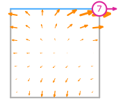
\(\displaystyle l_{7}:\boldsymbol{v}\mapsto\displaystyle\int_{e_{3}}\boldsymbol{v}\cdot(s_{0})\hat{\boldsymbol{t}}_{3}\)
where \(e_{3}\) is the 3rd edge;
\(\hat{\boldsymbol{t}}_{3}\) is the tangent to edge 3;
and \(s_{0},s_{1}\) is a parametrisation of \(e_{3}\).
\(\displaystyle \boldsymbol{\phi}_{7} = \left(\begin{array}{c}\displaystyle \frac{y \left(18 x y - 6 x - 3 y - 1\right)}{2}\\\displaystyle \frac{9 x \left(- 2 x y + x + 2 y - 1\right)}{2}\end{array}\right)\)
This DOF is associated with edge 3 of the reference element.
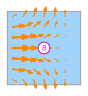
\(\displaystyle l_{8}:\mathbf{v}\mapsto\displaystyle\int_{R}\left(\begin{array}{c}\displaystyle 1\\\displaystyle 0\end{array}\right)\cdot\mathbf{v}\)
where \(R\) is the reference element.
\(\displaystyle \boldsymbol{\phi}_{8} = \left(\begin{array}{c}\displaystyle 3 y \left(6 x y - 6 x - 5 y + 5\right)\\\displaystyle 9 x \left(- 2 x y + x + 2 y - 1\right)\end{array}\right)\)
This DOF is associated with face 0 of the reference element.
where \(R\) is the reference element.
\(\displaystyle \boldsymbol{\phi}_{8} = \left(\begin{array}{c}\displaystyle 3 y \left(6 x y - 6 x - 5 y + 5\right)\\\displaystyle 9 x \left(- 2 x y + x + 2 y - 1\right)\end{array}\right)\)
This DOF is associated with face 0 of the reference element.
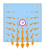
\(\displaystyle l_{9}:\mathbf{v}\mapsto\displaystyle\int_{R}\left(\begin{array}{c}\displaystyle 0\\\displaystyle -1\end{array}\right)\cdot\mathbf{v}\)
where \(R\) is the reference element.
\(\displaystyle \boldsymbol{\phi}_{9} = \left(\begin{array}{c}\displaystyle 9 y \left(2 x y - 2 x - y + 1\right)\\\displaystyle 3 x \left(- 6 x y + 5 x + 6 y - 5\right)\end{array}\right)\)
This DOF is associated with face 0 of the reference element.
where \(R\) is the reference element.
\(\displaystyle \boldsymbol{\phi}_{9} = \left(\begin{array}{c}\displaystyle 9 y \left(2 x y - 2 x - y + 1\right)\\\displaystyle 3 x \left(- 6 x y + 5 x + 6 y - 5\right)\end{array}\right)\)
This DOF is associated with face 0 of the reference element.
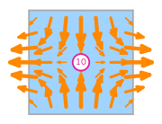
\(\displaystyle l_{10}:\mathbf{v}\mapsto\displaystyle\int_{R}\left(\begin{array}{c}\displaystyle s_{0}\\\displaystyle - s_{1}\end{array}\right)\cdot\mathbf{v}\)
where \(R\) is the reference element;
and \(s_{0},s_{1}\) is a parametrisation of \(R\).
\(\displaystyle \boldsymbol{\phi}_{10} = \left(\begin{array}{c}\displaystyle 18 y \left(- 2 x y + 2 x + y - 1\right)\\\displaystyle 18 x \left(2 x y - x - 2 y + 1\right)\end{array}\right)\)
This DOF is associated with face 0 of the reference element.